Herbaceous Production Report Methods

The herbaceous production report rapidly identifies deviations from historical averages. Two types of maps are provided: a national heat map for understanding general patterns and a county map for evaluating individual counties. Historical averages are provided as two different metrics: 1) a previous 10-year average, e.g., 2016-2025, representing the most recent trends in herbaceous production; and 2) a 30-year average, 1991-2020, representing the current climate standard normal established by the World Meteorological Organization. Counties can be selected to view and print a one-page production report specific to that county.

Data Processing

For each 16-day period, herbaceous production is calculated as the combined estimate of aboveground production for annual and perennial forbs and grasses (Jones et al. 2021). Deviations are defined as the percent difference between a long-term average and current 16-day herbaceous production.

Total herbaceous production is summed by 75x75km grid cells for the national heat map and by individual counties. The 75x75km grid cell size was selected to optimize map detail and load times. Lands identified as cropland, development, and water in the National Land Cover Database are excluded from the analysis.

Historical averages are calculated at the beginning of each new year. Grid cell and county totals are recalculated when the latest 16-day RAP production data become available.

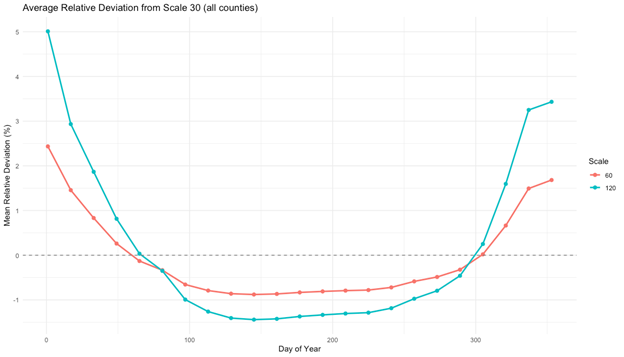
To make computations more efficient, herbaceous production totals are calculated using pyramid levels generated alongside 16-day RAP production data. All calculations utilize a resolution of 60x60m, equal to the first pyramid level and representing the mean value of the original 30x30m pixels contained therein. This approach substantially reduces the computation and cost of producing deviation maps, while minimizing errors associated with aggregation and the intersection with county boundaries, grid cells, and excluded land cover classes. The size of these errors (i.e., the difference between herbaceous production totals calculated at 30m vs. 60m resolution) varies throughout the year, with the smallest occurring at the peak of the growing season and the largest at the beginning and end of the calendar year when herbaceous production is typically low or non-existent (see Figure 1).

The Google Earth Engine script used to prepare map data can be viewed here.

Heat Maps

Heat maps are generated using the Contour mark of the Observable Plot JavaScript library. This function interpolates point samples to a continuous raster and then spatially bins raster values using the marching squares algorithm. For heat maps, x and y arguments of the function are set to the centroid coordinates of our 75x75km resolution grid in Albers equal-area conic projection. The “walk on spheres” algorithm described by Sawhney and Crane is used to interpolate herbaceous production deviation values between centroids. To improve interpretation, heat maps are simplified by smoothing interpolated values prior to applying marching squares using a “blur” radius of 4 pixels. Scott’s normal reference rule is used to dynamically compute contour (bin) thresholds each time a map is created.

References

Jones, M.O., N.P. Robinson, D.E. Naugle, J.D. Maestas, M.C. Reeves, R.W. Lankston, and B.W. Allred. 2021. Annual and 16-day rangeland production estimates for the western United States. Rangeland Ecology & Management 77:112–117. http://dx.doi.org/10.1016/j.rama.2021.04.003